Building a DC Power Flow Solver in Elixir: Nodes, Edges, and the B Matrix

On April 28th, 2025, Spain turned off. I mean that almost literally: the entire national power grid went down. No lights, no internet, no metro, no traffic lights, nothing. I was in a work meeting when everything turned off.

I remembered some of my friends from Uni studied Electrical Engineering, and they were making some kind of project to analyze power flow; I believe power flow estimates were in the heads of the ones trying to solve the problems that day. So a year or so later I got interested: How does one estimate the power flow in a grid?, How do you figure out how much is flowing through each line? How do you estimate when to generate more energy or lower it down a little?

I started reading about power flow estimates, simulations, specifically the PowerWorld program, which does this for you but at a bigger scale, and since I was learning Elixir, I started writing GridEx, a library for modeling power grids and solving the power flow problem in Elixir. This article walks through the primitives: the node, the edge, the topology, the schedule, and the solver itself.

---

What is power flow, and why DC?

A power grid has generators that inject electricity and loads (factories, homes, buildings) that consume it. Power flow analysis answers a concrete question: given who's producing and who's consuming, how much power is actually traveling through each transmission line?

The full AC power flow problem is nonlinear. It involves complex voltages, reactive power, and needs to be solved iteratively with something like Newton-Raphson. It's accurate, but it's also a lot. For many use cases (planning, quick analysis, simulation, learning, or post-blackout curiosity) you can use a simpler approximation that's still good enough.

The DC approximation makes three assumptions:

• Resistance in transmission lines is negligible; only reactance matters
• Voltage magnitudes at all buses are close to 1.0 per unit
• Angle differences between connected buses are small

With those in place, the relationship between power and angles becomes linear: P_ij = b_ij × (θ_i − θ_j), where b_ij is the susceptance of the line (1/reactance) and θ_i, θ_j are the voltage angles at each end. The whole thing is a linear system you can solve exactly.

---

Modeling the bus: GridEx.Node

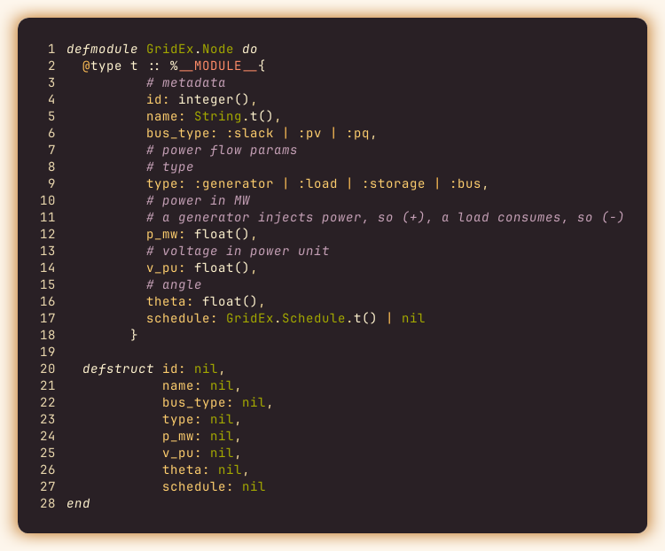
In power systems, a bus is an electrical connection point, where generators, loads, or lines meet. I modeled it as a Node struct.

A few design decisions worth unpacking.

bus_type can be :slack, :pv, or :pq. These are standard power systems classifications:

• :slack is the reference bus. Its angle is fixed at θ = 0 and it absorbs whatever power imbalance exists in the system. Every grid needs exactly one.
• :pv buses have a fixed voltage magnitude and a known real power injection, typically energy generators.
• :pq buses have known real and reactive power, typically loads. In the DC approximation we only care about real power, so in practice most non-slack nodes just need a p_mw.

p_mw follows a sign convention: positive means the node is injecting power (generator), negative means it's consuming power (load). The grid must balance, so the sum of all injections must be zero; the solver enforces this implicitly.

theta starts as nil. It's an output, not an input; the solver fills it in.

---

Modeling the line: GridEx.Edge

An edge is a transmission line connecting two buses.

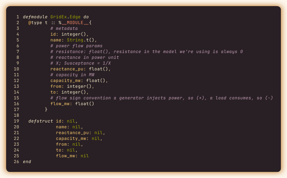
The commented-out resistance field is the DC approximation baked directly into the data model. It's not missing by accident; in this model, resistance is assumed zero, so there's no point storing it. What matters is reactance_pu, from which we get susceptance: b = 1 / reactance_pu. The higher the susceptance, the easier power flows through that line.

flow_mw is another output field, like theta on the node. It's nil until the solver writes in the result.

The from and to fields are plain node IDs. Keeping track of where these lines connect makes the topology easy to pass around and pattern-match later on. The capacity_mw is there for monitoring, the solver doesn't enforce it, but you'd use it to detect overloads or feed into an optimal power flow problem.

---

Assembling the graph: GridEx.Topology

The topology is deliberately minimal: a map of nodes and a map of edges, keyed by their IDs.

defmodule GridEx.Topology do
  @type t :: %__MODULE__{
          nodes: %{integer() => Node.t()},
          edges: %{integer() => Edge.t()}
        }

  defstruct nodes: %{}, edges: %{}
end

The topology flows through the whole pipeline as a plain struct, in from the caller, out with angles and flows populated. It's the single source of truth that every stage reads from and writes to.

---

Making it dynamic: GridEx.Schedule

Real grids don't sit still. Loads shift throughout the day (some even depending on sport events), solar generation follows the sun (if any), batteries charge and discharge on demand. I added a Schedule type to handle time-varying power injections on any node.

A schedule is a tagged union with three variants:

• {:constant, value}: same power every tick. Dead simple, useful for testing.
• {:sinusoidal, params}: oscillating load with amplitude, period, phase, and offset. Good for modeling daily consumption curves, wind generation, or the chaotic energy of a city waking up.
• {:piecewise, [{tick, value}, ...]}: a step function where the active value is the last defined breakpoint at or before the current tick. If you have measured data, you could use this to match it in a simulation.

Before the solver runs on each tick, Schedule.at(schedule, tick) is called to update the node's p_mw. The solver then sees the current injection and hands you off the result.

---

The solver: GridEx.PowerFlow.Dc

This is the core of the library. The full pipeline:

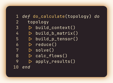
A Topology goes in, an updated Topology comes out. I love how Elixir's pipe operator makes this kind of pipeline read exactly like a description of the algorithm. Let me walk through each step.

Building the B matrix

The B matrix is an n×n susceptance matrix, the weighted Laplacian of the grid graph, where the weights are the susceptances of the transmission lines.

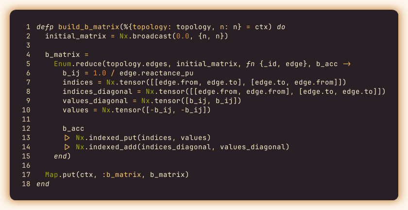
For each edge (i, j) with susceptance b_ij = 1 / reactance_pu:

• The off-diagonal entries B[i,j] and B[j,i] are set to −b_ij
• The diagonal entries B[i,i] and B[j,j] each get +b_ij added to them

The diagonal ends up holding the total susceptance connected to each bus, and the off-diagonal entries encode which buses are connected and how easily power flows between them.

Reducing and solving

Before solving, we remove the slack bus from the system. Since θ = 0 at the slack by definition, it has no unknowns; its row and column can be sliced out entirely.

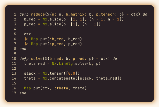
Then Nx.LinAlg.solve(b_red, p_red) solves B_red × θ_red = P_red; that one line is doing all the heavy lifting. After that, we prepend 0.0 to reconstruct the full angle vector with the slack included.

Computing flows and writing back

With angles computed, flows are one formula per edge: P_ij = b_ij × (θ_i − θ_j). The final step writes all the computed thetas back into the node structs and all the computed flows back into the edge structs, returning the updated Topology.

The whole pipeline is pure and stateless. Same topology in, same result out.

---

Running it in time: GridEx.SimulationServer

The solver is a pure function: topology in, topology out. The GenServer is what adds the time dimension.

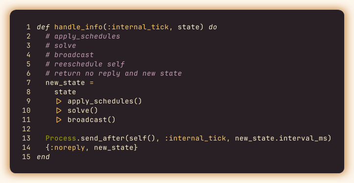
Every tick, handle_info(:internal_tick, state) does three things:

1. Apply schedules: updates each node's p_mw for the current tick given the configured Schedule
2. Solve: runs the DC solver on the updated topology
3. Broadcast: pushes the result to Phoenix PubSub so any subscriber (a LiveView, a logger, a monitoring process) can react

Then it reschedules itself.

This pattern maps beautifully to the domain. A power grid simulation is a process that holds state and updates it on a clock. The tick counter becomes time, the topology becomes the simulation state, and PubSub lets any number of consumers react without the simulation server knowing or caring about any of them. Elixir really does feel like it was made for this kind of thing.

---

What's next

GridEx is still early. The obvious next step is an AC solver, Newton-Raphson or fast-decoupled, which would make voltage magnitudes and reactive power meaningful. Beyond that: contingency analysis (what happens to flows when a line trips?), a LiveView visualization of the topology in real time, and eventually optimal power flow to find the minimum-cost dispatch. I'd also like to benchmark it against PowerWorld, and why not, even a Topology builder to teach this kind of stuff to future engineers.

The DC solver is a solid foundation for all of that and it has made me study the field and test out some topologies already to see it all working correctly. Linear, fast, and exact within the approximation.